Warm-up: Network analysis with Python
Mediterranean School of Complex Networks (MSCX) 2022 - Catania, Italy
Python
What is python
Python is an interpreted, object-oriented, high-level programming language with dynamic semantics. […]
It is suitable for rapid development and for use as a “glue language” to connect various components (e.g., written in different languages).
Python is one of the most used programming languages[1]
[1]: StackOverflow’s 2021 survey
Why is python so popular?
Its popularity can be rooted to its characteristics
- Python is fast to learn, very versatile and flexible
- It is very high-level, and complex operations can be performed with few lines of code
And to its large user-base:
- Vast assortment of libraries
- Solutions to your problems may be already available (e.g., on StackOverflow)
Some real-world applications
- Data science (loading, processing and plotting of data)
- Scientific and Numeric computing
- Modeling and Simulation
- Web development
- Artificial Intelligence and Machine Learning
- Image and Text processing
- Scripting
How to get python?
Using the default environment that comes with your OS is not a great idea:
- Usually older python versions are shipped
- You cannot upgrade the python version or the libraries freely
- Some functions of your OS may depend on it
You can either:
- Download python
- Use a distribution like Anaconda
Anaconda
Anaconda is a python distribution that packs the most used libraries for data analysis, processing and visualization
Anaconda installations are managed through the conda package manager
Anaconda “distribution” is free and open source

Python virtual environments
A virtual environment is a Python environment such that the Python interpreter, libraries and scripts installed into it are isolated from those installed in other virtual environments
Environments are used to freeze specific interpreter and libraries versions for your projects
If you start a new project and need newer libraries, just create a new environment
You won’t have to worry about breaking the other projects
Environment creation
conda create –name <ENV_NAME> [<PACKAGES_LIST>] [–channel
]
You can also specify additional channels to search for packages (in order)
Example:
conda create –name gt python=3.9 graph-tool pytorch torchvision torchaudio cudatoolkit=11.3 pyg seaborn numpy scipy matplotlib jupyter -c pyg -c pytorch -c nvidia -c anaconda -c conda-forge
Switch environment
conda activate <ENV_NAME>
Example
conda activate gt
Data analysis and visualization libraries
- NumPy
- SciPy
- Matplotlib
- Seaborn
- Pandas
These libraries are general, and can be used also in Network Analysis
Network analysis and visualization libraries
- graph-tool
- PyTorch Geometric (PyG)
NumPy
NumPy is the fundamental package for scientific computing in Python.
NumPy offers new data structures:
- Multidimensional array objects (the ndarray)
- Various derived objects (like masked arrays)
And also a vast assortment of functions:
- Mathematical functions (arithmetic, trigonometric, hyperbolic, rounding, …)
- Sorting, searching, and counting
- Operations on Sets
- Input and output
- Fast Fourier Transform
- Complex numbers handing
- (pseudo) random number generation
NumPy is fast:
- Its core is written in C/C++
- Arrays are stored in contiguous memory locations
It also offers tools for integrating C/C++ code
Many libraries are built on top of NumPy’s arrays and functions.
The ndarray
| Mono-dimensional | Multi-dimensional |
|---|---|
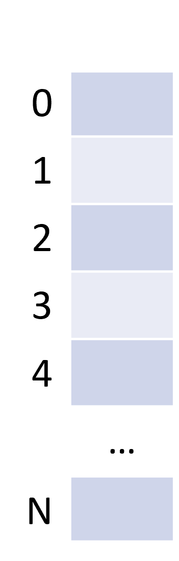 | 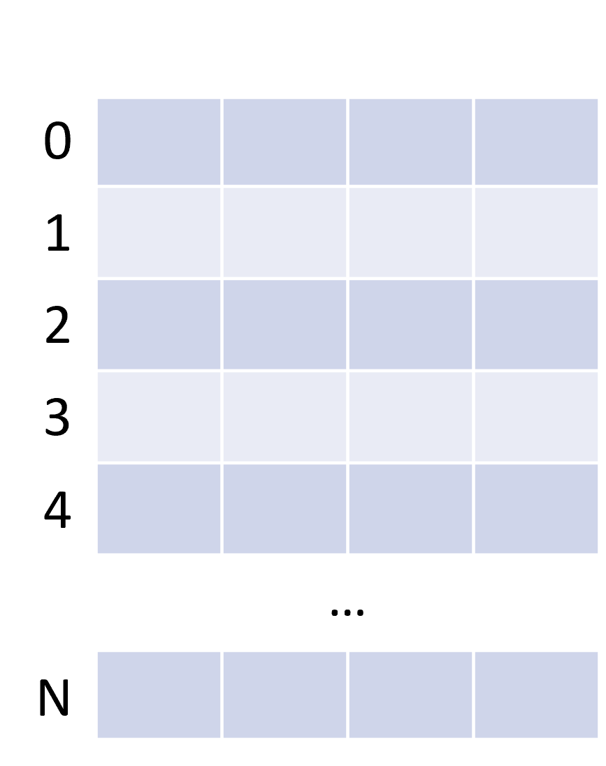 |
import numpy as np
np.random.rand(3)
array([0.23949294, 0.49364534, 0.10055484])
np.random.rand(1, 3)
array([[0.45292492, 0.32975629, 0.53797728]])
np.random.randint(10, size=(2, 2, 2))
array([[[9, 1],
        [9, 9]],

       [[5, 7],
        [3, 3]]])
SciPy
SciPy is a collection of mathematical algorithms and convenience functions built on the NumPy library
SciPy is written in C and Fortran, and provides:
- Algorithms for optimization, integration, interpolation, eigenvalue problems, algebraic equations, differential equations, statistics, etc.
- Specialized data structures, such as sparse matrices and k-dimensional trees
- Tools for the interactive Python sessions
SciPy’s main subpackages include:
Data clustering algorithms
Physical and mathematical constants
Fast Fourier Transform routines
Integration and ordinary differential equation solvers
Linear algebra
…
…
N-dimensional image processing
Optimization and root-finding routines
Signal processing
Sparse matrices and associated routines
Spatial data structures and algorithms
Statistical distributions and functions
import scipy as sp
Sparse matrices
There are many sparse matrices implementations, each optimized for different operations.
For instance:
- Coordinate (COO)
- Linked List Matrix (LIL)
- Compressed Sparse Row (CSR)
- Compressed Sparse Column (CSC)
Check this nice tutorial for more! Sparse matrices tutorial
Pandas
pandas allows easy data organization, filtering, analysis and plotting
pandas provides data structures for “relational” or “labeled” data, for instance:
- Tabular data with heterogeneously-typed columns, as in an Excel spreadsheet
- Ordered and unordered time series data
- Arbitrary matrix data (even heterogeneous typed) with row and column labels
The two primary data structures provided are the:
- Series (1-dimensional)
- DataFrame (2-dimensional)
| Series | DataFrame |
|---|---|
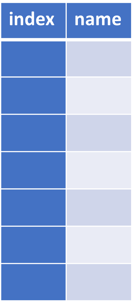 | 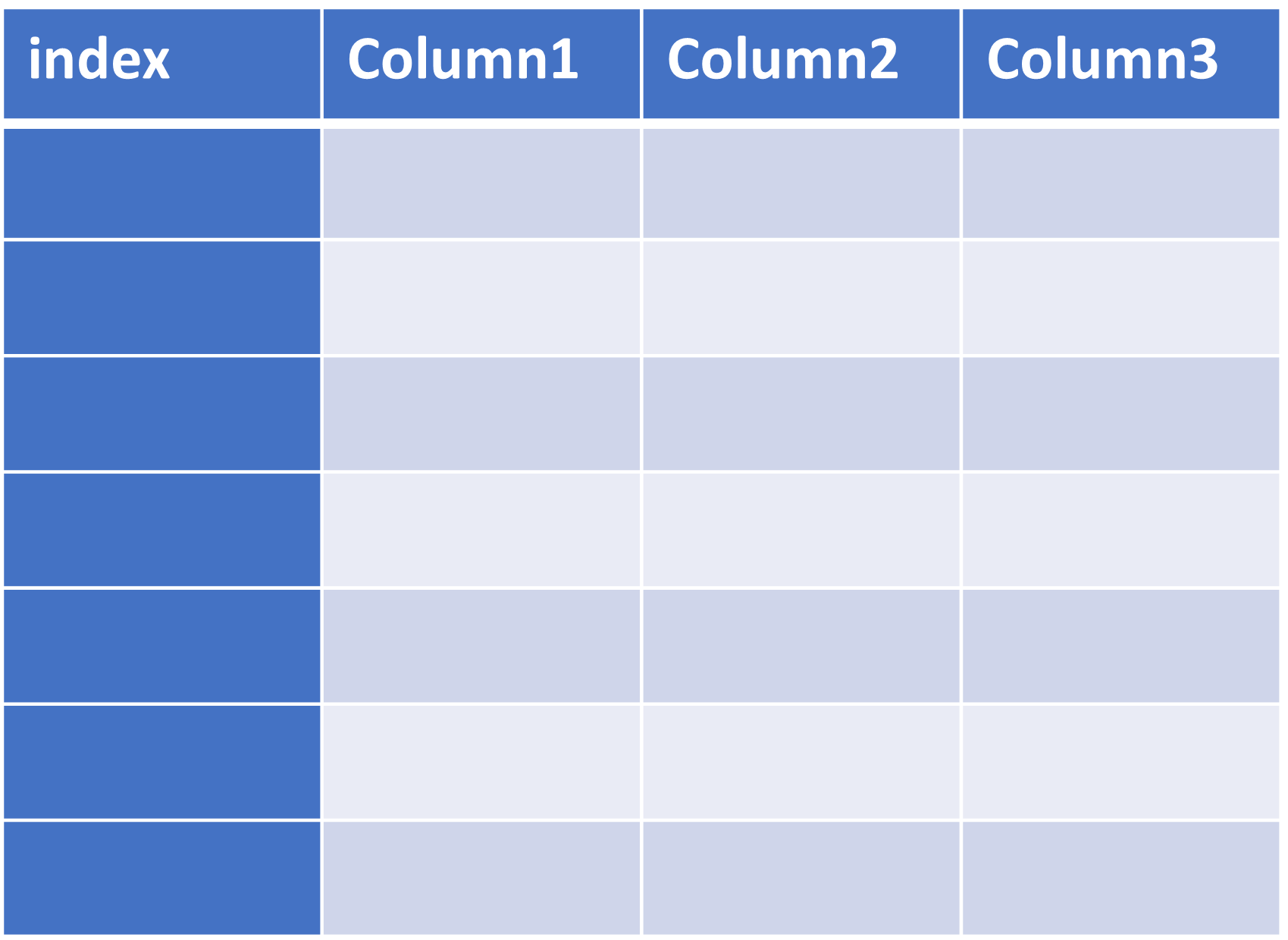 |
These structures heavily rely on NumPy and its arrays
pandas integrates well with other libraries built on top of NumPy
Supported file formas
pandas can recover data from/store data to SQL databases, Excel, CSVs…

import pandas as pd
DataFrame example
Penguins example dataset from the Seaborn package
penguins = sns.load_dataset("penguins")
display(penguins)
| species | island | bill_length_mm | bill_depth_mm | flipper_length_mm | body_mass_g | sex | |
|---|---|---|---|---|---|---|---|
| 0 | Adelie | Torgersen | 39.1 | 18.7 | 181.0 | 3750.0 | Male |
| 1 | Adelie | Torgersen | 39.5 | 17.4 | 186.0 | 3800.0 | Female |
| 2 | Adelie | Torgersen | 40.3 | 18.0 | 195.0 | 3250.0 | Female |
| 3 | Adelie | Torgersen | NaN | NaN | NaN | NaN | NaN |
| 4 | Adelie | Torgersen | 36.7 | 19.3 | 193.0 | 3450.0 | Female |
| ... | ... | ... | ... | ... | ... | ... | ... |
| 339 | Gentoo | Biscoe | NaN | NaN | NaN | NaN | NaN |
| 340 | Gentoo | Biscoe | 46.8 | 14.3 | 215.0 | 4850.0 | Female |
| 341 | Gentoo | Biscoe | 50.4 | 15.7 | 222.0 | 5750.0 | Male |
| 342 | Gentoo | Biscoe | 45.2 | 14.8 | 212.0 | 5200.0 | Female |
| 343 | Gentoo | Biscoe | 49.9 | 16.1 | 213.0 | 5400.0 | Male |
344 rows × 7 columns
Series of the species
penguins["species"]
0      Adelie
1      Adelie
2      Adelie
3      Adelie
4      Adelie
        ...
339    Gentoo
340    Gentoo
341    Gentoo
342    Gentoo
343    Gentoo
Name: species, Length: 344, dtype: object
Unique species
penguins["species"].unique()
array(['Adelie', 'Chinstrap', 'Gentoo'], dtype=object)
Average bill length
penguins["bill_length_mm"].mean()
43.9219298245614
Standard deviation of the bill length
penguins["bill_length_mm"].std()
5.4595837139265315
Data filtering for male penguins
penguins["sex"] == "Male"
0       True
1      False
2      False
3      False
4      False
       ...
339    False
340    False
341     True
342    False
343     True
Name: sex, Length: 344, dtype: bool
penguins.loc[                         # .loc property
    penguins["sex"] == "Male"         # Row filter (boolean)
]
| species | island | bill_length_mm | bill_depth_mm | flipper_length_mm | body_mass_g | sex | |
|---|---|---|---|---|---|---|---|
| 0 | Adelie | Torgersen | 39.1 | 18.7 | 181.0 | 3750.0 | Male |
| 5 | Adelie | Torgersen | 39.3 | 20.6 | 190.0 | 3650.0 | Male |
| 7 | Adelie | Torgersen | 39.2 | 19.6 | 195.0 | 4675.0 | Male |
| 13 | Adelie | Torgersen | 38.6 | 21.2 | 191.0 | 3800.0 | Male |
| 14 | Adelie | Torgersen | 34.6 | 21.1 | 198.0 | 4400.0 | Male |
| ... | ... | ... | ... | ... | ... | ... | ... |
| 333 | Gentoo | Biscoe | 51.5 | 16.3 | 230.0 | 5500.0 | Male |
| 335 | Gentoo | Biscoe | 55.1 | 16.0 | 230.0 | 5850.0 | Male |
| 337 | Gentoo | Biscoe | 48.8 | 16.2 | 222.0 | 6000.0 | Male |
| 341 | Gentoo | Biscoe | 50.4 | 15.7 | 222.0 | 5750.0 | Male |
| 343 | Gentoo | Biscoe | 49.9 | 16.1 | 213.0 | 5400.0 | Male |
168 rows × 7 columns
Average bill length for male penguins
penguins.loc[ penguins["sex"] == "Male",   # Mask (row filter)
              "bill_length_mm",            # Column filter
].mean()
45.85476190476191
Average bill length and weight for female penguins
penguins.loc[penguins["sex"] == "Female",                # Mask (row filter)
             ["bill_length_mm", "body_mass_g"]           # Column filter
            ].mean()
bill_length_mm      42.096970
body_mass_g       3862.272727
dtype: float64
Matplotlib
Matplotlib is a comprehensive library for creating static, animated, and interactive visualizations in Python
Some plot examples
From the Matplotlib gallery
Line plots
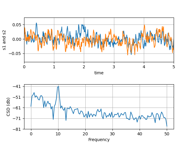
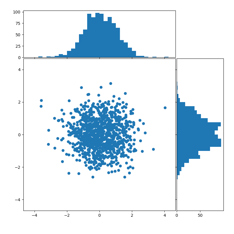
Scatterplots and histograms
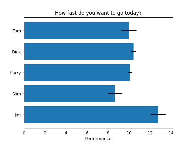
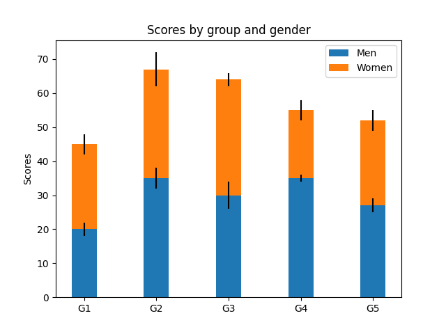
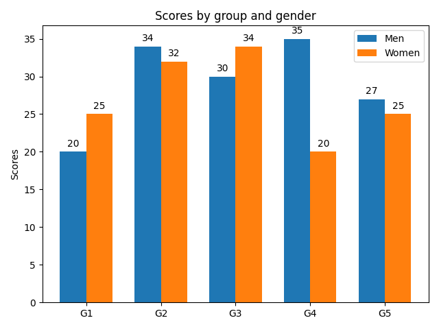
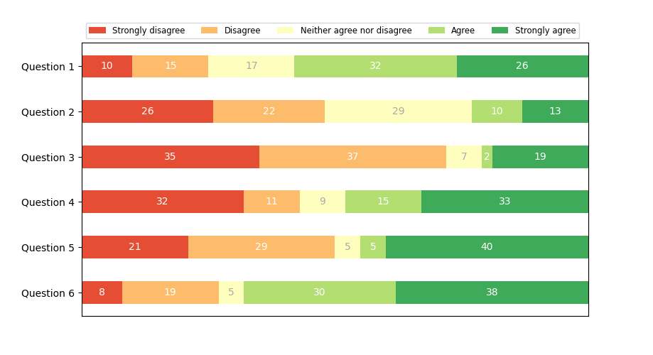
Barplots
Simple barplot
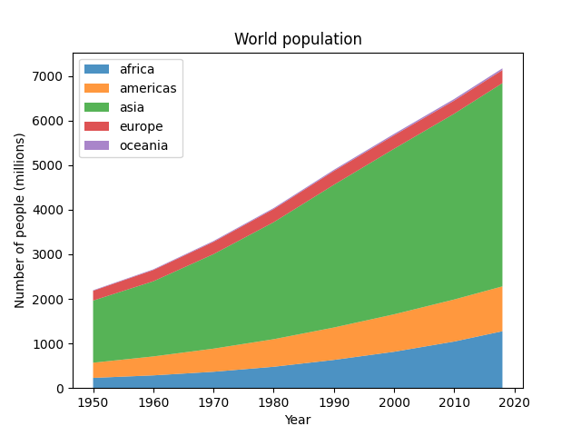
Stacked barplot
Grouped barplot
Horizontal bar chart
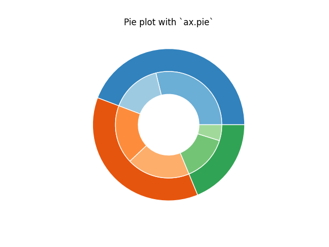
(Nested) pie charts
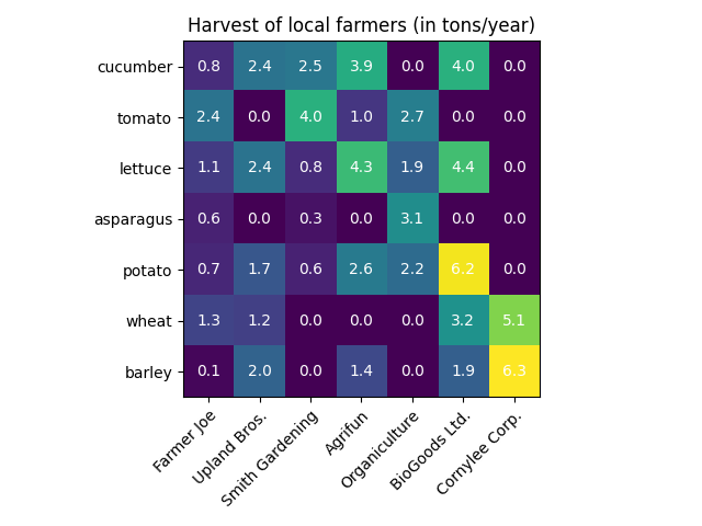
Heatmaps
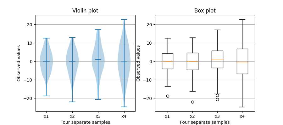
Violin and box plots
Stackplots
… and many more
import matplotlib.pyplot as plt
Seaborn
Seaborn is a library for making statistical graphics in Python
Thanks to its high-level interface, it makes plotting very complex figures easy
Seaborn builds on top of matplotlib and integrates closely with pandas data structures
import seaborn as sns
It provides helpers to improve how all matplotlib plots look:
- Theme and style
- Colors (even colorblind palettes)
- Scaling, to quickly switch between presentation contexts (e.g., plot, poster and talk)
sns.reset_defaults()
plt.plot(range(10), range(10))
[<matplotlib.lines.Line2D at 0x7f1ed75972b0>]
sns.set_theme(context="talk",
              style="ticks",
              palette="deep",
              font="sans-serif",
#               font_scale=1,
              color_codes=True,
              rc={
                  'figure.facecolor': 'white'
#                   'figure.figsize': (10, 6),
#                   "text.usetex": True,
#                   "font.family": "sans-serif",
              },

              )
plt.plot(range(10), range(10))
sns.despine()
Seaborn’s FacetGrid offers a convenient way to visualize multiple plots in grids
They can be drawn with up to three dimensions: rows, columns and hue
Tutorial: Building structured multi-plot grids
penguins.head()
| species | island | bill_length_mm | bill_depth_mm | flipper_length_mm | body_mass_g | sex | |
|---|---|---|---|---|---|---|---|
| 0 | Adelie | Torgersen | 39.1 | 18.7 | 181.0 | 3750.0 | Male |
| 1 | Adelie | Torgersen | 39.5 | 17.4 | 186.0 | 3800.0 | Female |
| 2 | Adelie | Torgersen | 40.3 | 18.0 | 195.0 | 3250.0 | Female |
| 3 | Adelie | Torgersen | NaN | NaN | NaN | NaN | NaN |
| 4 | Adelie | Torgersen | 36.7 | 19.3 | 193.0 | 3450.0 | Female |
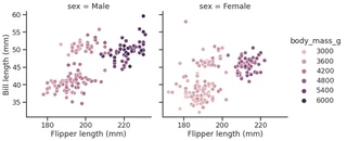
g = sns.relplot(data=penguins,
                x="flipper_length_mm",
                y="bill_length_mm",
                col="sex",
                hue="body_mass_g"
               )
g.set_axis_labels("Flipper length (mm)", "Bill length (mm)")
<seaborn.axisgrid.FacetGrid at 0x7f1ed7597a90>
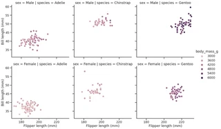
g = sns.relplot(data=penguins,
                x="flipper_length_mm",
                y="bill_length_mm",
                row="sex",
                col="species",
                hue="body_mass_g"
               )
g.set_axis_labels("Flipper length (mm)", "Bill length (mm)")
<seaborn.axisgrid.FacetGrid at 0x7f1ed73a5f10>
Some more plot examples
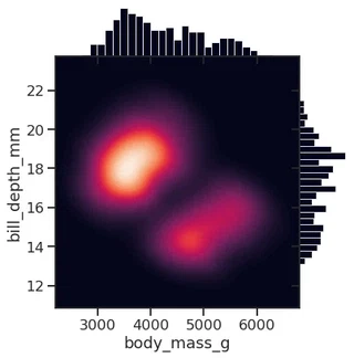
Smooth kernel density with marginal histograms (source)
g = sns.JointGrid(data=penguins, x="body_mass_g", y="bill_depth_mm", space=0)
g.plot_joint(sns.kdeplot,
             fill=True, clip=((2200, 6800), (10, 25)),
             thresh=0, levels=100, cmap="rocket")
g.plot_marginals(sns.histplot, color="#03051A", alpha=1, bins=25)
<seaborn.axisgrid.JointGrid at 0x7f1ed5671ca0>
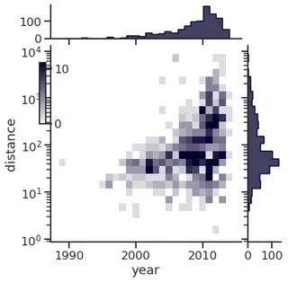
Joint and marginal histograms
g = sns.JointGrid(data=planets, x="year", y="distance", marginal_ticks=True)

# Set a log scaling on the y axis
g.ax_joint.set(yscale="log")

# Create an inset legend for the histogram colorbar
cax = g.figure.add_axes([.15, .55, .02, .2])

# Add the joint and marginal histogram plots
g.plot_joint(
    sns.histplot, discrete=(True, False),
    cmap="light:#03012d", pmax=.8, cbar=True, cbar_ax=cax
)
g.plot_marginals(sns.histplot, element="step", color="#03012d")
<seaborn.axisgrid.JointGrid at 0x7f1ed4503c70>
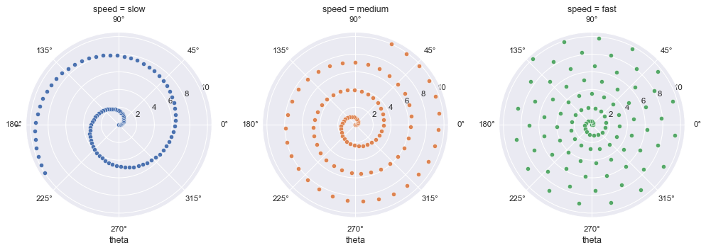
Custom projections
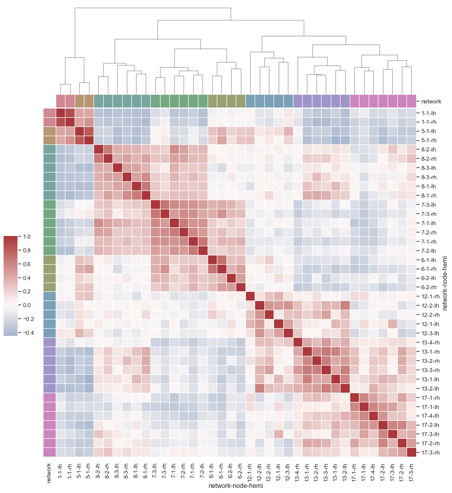
Discovering structure in heatmap data
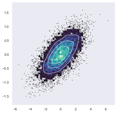
Bivariate plot with multiple elements
Network Analysis with Python
Three main libraries:
- graph-tool
- networkx
- python-igraph
graph-tool
graph-tool is a graph analysis library for Python
It provides the Graph data structure, and various algorithms
It is mostly written in C++, and based on the Boost Graph Library
It supports multithreading and it is fairly easy to extend
Built in algorithms:
- Topology analysis tools
- Centrality-related algorithms
- Clustering coefficient (transitivity) algorithms
- Correlation algorithms, like the assortativity
- Dynamical processes (e.g., SIR, SIS, …)
- Graph drawing tools
- Random graph generation
- Statistical inference of generative network models
- Spectral properties computation
import graph_tool.all as gt
Performance comparison (source: graph-tool.skewed.de/)
| Algorithm | graph-tool (16 threads) | graph-tool (1 thread) | igraph | NetworkX |
|---|---|---|---|---|
| Single-source shortest path | 0.0023 s | 0.0022 s | 0.0092 s | 0.25 s |
| Global clustering | 0.011 s | 0.025 s | 0.027 s | 7.94 s |
| PageRank | 0.0052 s | 0.022 s | 0.072 s | 1.54 s |
| K-core | 0.0033 s | 0.0036 s | 0.0098 s | 0.72 s |
| Minimum spanning tree | 0.0073 s | 0.0072 s | 0.026 s | 0.64 s |
| Betweenness | 102 s (~1.7 mins) | 331 s (~5.5 mins) | 198 s (vertex) + 439 s (edge) (~ 10.6 mins) | 10297 s (vertex) 13913 s (edge) (~6.7 hours) |
How to load a network
Choose a graph analysis library. The right one mostly depends on your needs (e.g., functions, performance, etc.)
In this warm-up, we will use graph-tool.
To load the network, we need to use the right loader function, which depends on the file format
File formats
Many ways to represent and store graphs.
The most popular ones are:
- edgelist
- GraphML
For more about file types, check the NetworkX documentation
Edgelist (.el, .edge, …)
As the name suggests, it is a list of node pairs (source, target) and edge properties (if any). Edgelists cannot store any information about the nodes, or about the graph (not even about the directedness)
Values may be separated by commas, spaces, tabs, etc. Comments may be supported by the reader function.
Example file:
# source, target, weight
0,1,1
0,2,2
0,3,2
0,4,1
0,5,1
0,6,1
1,18,1
1,3,1
1,4,2
2,0,1
2,25,1
#...
GraphML (.graphml, .xml)
Flexible format based on XML.
It can store hierarchical graphs, information (i.e., attributes or properties) about the graph, the nodes and the edges.
Main drawback: heavy disk usage (space, and I\O time)
Example of the file:
<?xml version="1.0" encoding="UTF-8"?>
<graphml xmlns="http://graphml.graphdrawing.org/xmlns"
xmlns:xsi="http://www.w3.org/2001/XMLSchema-instance"
xsi:schemaLocation="http://graphml.graphdrawing.org/xmlns http://graphml.graphdrawing.org/xmlns/1.0/graphml.xsd">
<!-- property keys -->
<key id="key0" for="node" attr.name="_pos" attr.type="vector_float" />
<key id="key1" for="graph" attr.name="citation" attr.type="string" />
<key id="key2" for="graph" attr.name="description" attr.type="string" />
<!-- [...] -->
<key id="key8" for="edge" attr.name="weight" attr.type="short" />
<graph id="G" edgedefault="directed" parse.nodeids="canonical" parse.edgeids="canonical" parse.order="nodesfirst">
<!-- graph properties -->
<data key="key1">['J. S. Coleman. "Introduction to Mathematical Sociology." London Free Press Glencoe (1964), http://www.abebooks.com/Introduction-Mathematical-Sociology-COLEMAN-James-S/189127582/bd']</data>
<data key="key2">A network of friendships among male students in a small high school in Illinois from 1958. An arc points from student i to student j if i named j as a friend, in either of two identical surveys (from Fall and Spring semesters). Edge weights are the number of surveys in which the friendship was named.</data>
<!-- [...] -->
<!-- vertices -->
<node id="n0">
<data key="key0">0.92308158331278289, 12.186082864409657</data>
</node>
<node id="n1">
<data key="key0">1.2629064355495019, 12.213213242633238</data>
</node>
<node id="n2">
<data key="key0">1.1082744694986855, 12.190211909578192</data>
</node>
<!-- [...] -->
<!-- edges -->
<edge id="e0" source="n0" target="n1">
<data key="key8">1</data>
</edge>
<edge id="e1" source="n0" target="n2">
<data key="key8">2</data>
</edge>
<edge id="e2" source="n0" target="n3">
<data key="key8">2</data>
</edge>
<edge id="e3" source="n0" target="n4">
<data key="key8">1</data>
</edge>
<!-- [...] -->
</graph>
</graphml>
How to load a network
Choose a graph analysis library. The right one mostly depends on your needs (e.g., features, performance, etc.)
In this warm-up, we will use graph-tool.
To load the network, we need to use the right loader function, which depends on the file format
After identifying the file format and the right loader function, we load the network
g = gt.load_graph("highschool.graphml")

display(g)
<Graph object, directed, with 70 vertices and 366 edges, 1 internal vertex property, 1 internal edge property, 7 internal graph properties, at 0x7f1ed41879d0>
display(g.graph_properties)
{'citation': <GraphPropertyMap object with value type 'string', for Graph 0x7f1ed41879d0, at 0x7f1ed4187220>, 'description': <GraphPropertyMap object with value type 'string', for Graph 0x7f1ed41879d0, at 0x7f1ed4187130>, 'konect_meta': <GraphPropertyMap object with value type 'string', for Graph 0x7f1ed41879d0, at 0x7f1ed4187070>, 'konect_readme': <GraphPropertyMap object with value type 'string', for Graph 0x7f1ed41879d0, at 0x7f1ed41b80a0>, 'name': <GraphPropertyMap object with value type 'string', for Graph 0x7f1ed41879d0, at 0x7f1ed4225070>, 'tags': <GraphPropertyMap object with value type 'vector<string>', for Graph 0x7f1ed41879d0, at 0x7f1ed4225040>, 'url': <GraphPropertyMap object with value type 'string', for Graph 0x7f1ed41879d0, at 0x7f1ed4256d00>}
display(g.vertex_properties)
{'_pos': <VertexPropertyMap object with value type 'vector<double>', for Graph 0x7f1ed41879d0, at 0x7f1ed4187730>}
display(g.edge_properties)
{'weight': <EdgePropertyMap object with value type 'int16_t', for Graph 0x7f1ed41879d0, at 0x7f1ed4291130>}
Some network analysis
Get the number of nodes
number_of_nodes = g.num_vertices()
display(f"Number of nodes: {number_of_nodes}")
'Number of nodes: 70'
Get the number of edges
number_of_edges = g.num_edges()
display(f"Number of edges: {number_of_edges}")
'Number of edges: 366'
Get the in and out degrees
in_degree = g.get_in_degrees(g.get_vertices(), eweight=None)
average_in_degree = np.mean(in_degree)

display("Average in degree", average_in_degree)
'Average in degree'


5.228571428571429
out_degree = g.get_out_degrees(g.get_vertices(), eweight=None)
average_out_degree = np.mean(out_degree)
display("Average out degree", average_out_degree)
'Average out degree'


5.228571428571429
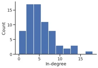
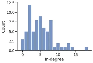
In-degree distribution
p = plt.hist(in_degree)

plt.ylabel("Count")
plt.xlabel("In-degree")
sns.despine()
p = sns.histplot(in_degree,
                 stat="count",
                 discrete=True,
)
p.set_xlabel("In-degree")
sns.despine()
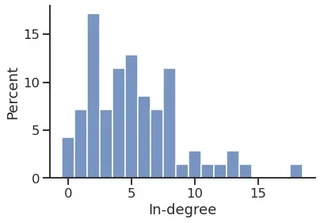
p = sns.histplot(in_degree,
             stat="percent",
             discrete=True,
)
p.set_xlabel("In-degree")
sns.despine()
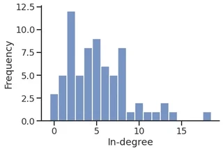
sns.histplot(in_degree,
             stat="frequency",
             discrete=True,
)
plt.xlabel("In-degree")
sns.despine()
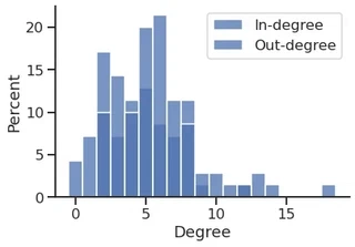
sns.histplot(in_degree,
             stat="percent",
             discrete=True,
             label="In-degree",
             legend=True,

)
sns.histplot(out_degree,
             stat="percent",
             discrete=True,
             label="Out-degree",
             legend=True,
)

plt.xlabel("Degree")
plt.legend()
sns.despine()
cmap = sns.color_palette("deep", n_colors=2)

cmap
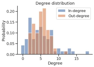
sns.histplot(in_degree,
             stat="probability",
             discrete=True,
             label="In-degree",
             legend=True,
             color=cmap[0],
             alpha=0.6,
)
sns.histplot(out_degree,
             stat="probability",
             discrete=True,
             label="Out-degree",
             legend=True,
             color=cmap[1],
             alpha=0.6,
)

plt.title("Degree distribution")
plt.xlabel("Degree")
plt.legend()
sns.despine()
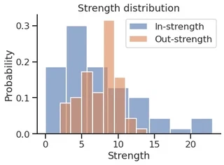
Get the in and out strength
weight = g.edge_properties["weight"]

in_strength = g.get_in_degrees(g.get_vertices(), eweight=weight)

out_strength = g.get_out_degrees(g.get_vertices(), eweight=weight)
sns.histplot(in_strength,
             stat="probability",
             discrete=False,
             label="In-strength",
             legend=True,
             color=cmap[0],
             alpha=0.6,
)

sns.histplot(out_strength,
             stat="probability",
             discrete=False,
             label="Out-strength",
             legend=True,
             color=cmap[1],
             alpha=0.6,
)

plt.title("Strength distribution")
plt.xlabel("Strength")
plt.legend()
sns.despine()
Store the values as a DataFrame
df = pd.DataFrame(
    data={
        ("Degree", "In"): in_degree,
        ("Degree", "Out"): out_degree,

        ("Strength", "In"): in_strength,
        ("Strength", "Out"): out_strength,
    },
)

df.head()
| Degree | Strength | |||
|---|---|---|---|---|
| In | Out | In | Out | |
| 0 | 2 | 6 | 2 | 8 |
| 1 | 2 | 3 | 3 | 4 |
| 2 | 2 | 4 | 3 | 5 |
| 3 | 12 | 6 | 19 | 9 |
| 4 | 13 | 5 | 21 | 9 |
… and plot the DF using Seaborn
melted_df = pd.melt(df, var_name=["Kind", "Direction"], value_name="Value")

melted_df
| Kind | Direction | Value | |
|---|---|---|---|
| 0 | Degree | In | 2.0 |
| 1 | Degree | In | 2.0 |
| 2 | Degree | In | 2.0 |
| 3 | Degree | In | 12.0 |
| 4 | Degree | In | 13.0 |
| ... | ... | ... | ... |
| 275 | Strength | Out | 7.0 |
| 276 | Strength | Out | 10.0 |
| 277 | Strength | Out | 10.0 |
| 278 | Strength | Out | 4.0 |
| 279 | Strength | Out | 5.0 |
280 rows × 3 columns
facet = sns.displot(melted_df,
                    x="Value",
                    kind="hist",
                    row="Kind",
                    col="Direction",
                    hue="Direction",
                    )
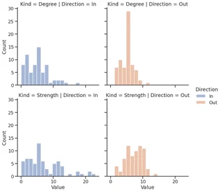
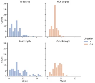
melted_df["Kind"] = melted_df["Kind"].apply(str.lower)

facet = sns.displot(melted_df,
                    x="Value",
                    kind="hist",
                    row="Kind",
                    col="Direction",
                    hue="Direction",
                    )

facet.set_titles(template="{col_name}-{row_name}")
<seaborn.axisgrid.FacetGrid at 0x7f1ecf5c6610>
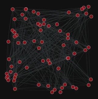
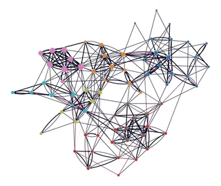
Graph visualization
1. Compute the node layout
pos = gt.fruchterman_reingold_layout(g, n_iter=1000)
2. Plot the network
gt.graph_draw(g, pos=pos,
              bg_color="#111",
              )
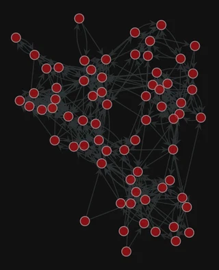
<VertexPropertyMap object with value type 'vector<double>', for Graph 0x7f1ed41879d0, at 0x7f1ed41312b0>
Add the edge weight
gt.graph_draw(g,
              pos=pos,
              edge_pen_width=g.edge_properties["weight"],
              bg_color="#111",
              )
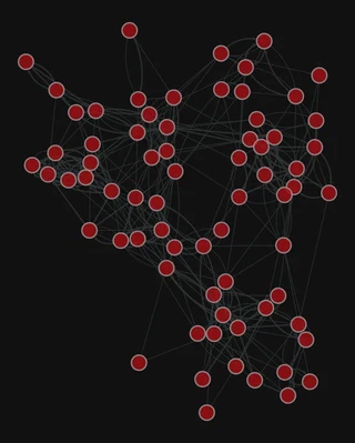
<VertexPropertyMap object with value type 'vector<double>', for Graph 0x7f1ed41879d0, at 0x7f1ecf79e910>
More layouts
pos = gt.sfdp_layout(g)

gt.graph_draw(g, pos=pos,
              edge_pen_width=g.edge_properties["weight"],
              bg_color="#111",
              )
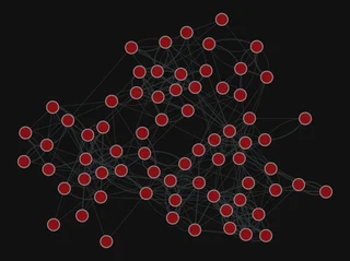
<VertexPropertyMap object with value type 'vector<double>', for Graph 0x7f1ed41879d0, at 0x7f1ecf79eca0>
pos = gt.arf_layout(g)

gt.graph_draw(g,
              pos=pos,
              bg_color="#111",
              )
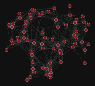
<VertexPropertyMap object with value type 'vector<double>', for Graph 0x7f1ed41879d0, at 0x7f1ed411b9a0>
pos = gt.random_layout(g)

gt.graph_draw(g,
              pos=pos,
              edge_pen_width=g.edge_properties["weight"],
              bg_color="#111",
              )
<VertexPropertyMap object with value type 'vector<double>', for Graph 0x7f1ed41879d0, at 0x7f1ecf645ac0>
Centrality computation
gw = gt.GraphView(g, vfilt=gt.label_largest_component(g))
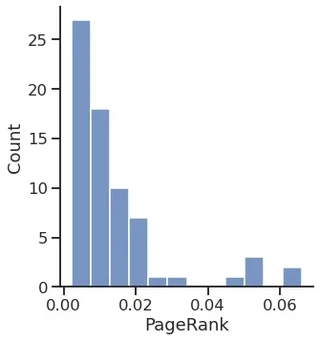
PageRank
pr = gt.pagerank(g)
sns.displot(pr.a)
plt.xlabel("PageRank")
Text(0.5, 15.439999999999998, 'PageRank')
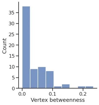
Betweenness
vertex_betweenness, edge_betweenness = gt.betweenness(g)
sns.displot(vertex_betweenness.a)
plt.xlabel("Vertex betweenness")
Text(0.5, 15.439999999999998, 'Vertex betweenness')
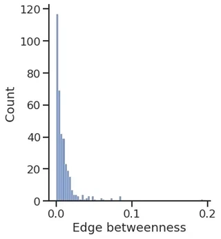
sns.displot(edge_betweenness.a)
plt.xlabel("Edge betweenness")
Text(0.5, 15.439999999999998, 'Edge betweenness')
gt.graph_draw(gw,
              pos=g.vp["_pos"],
              vertex_fill_color=pr, vorder=pr,
              edge_color=edge_betweenness,
              vertex_size=gt.prop_to_size(pr, mi=5, ma=15),
              vcmap=sns.color_palette("gist_heat", as_cmap=True),
              ecmap=sns.color_palette("rocket", as_cmap=True),
              edge_pen_width=g.edge_properties["weight"],
              bg_color="white",
              )
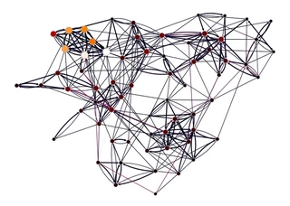
<VertexPropertyMap object with value type 'vector<double>', for Graph 0x7f1ed4113fa0, at 0x7f1ed40db340>
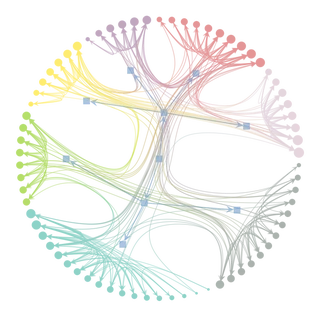
Inferring modular structure
# state = gt.minimize_blockmodel_dl(g)
state = gt.minimize_nested_blockmodel_dl(g)
state.draw()
(<VertexPropertyMap object with value type 'vector<double>', for Graph 0x7f1ed41879d0, at 0x7f1ecf7d77c0>,
 <GraphView object, directed, with 80 vertices and 79 edges, edges filtered by (<EdgePropertyMap object with value type 'bool', for Graph 0x7f1ecf32dfa0, at 0x7f1ecf338040>, False), vertices filtered by (<VertexPropertyMap object with value type 'bool', for Graph 0x7f1ecf32dfa0, at 0x7f1ecf330ee0>, False), at 0x7f1ecf32dfa0>,
 <VertexPropertyMap object with value type 'vector<double>', for Graph 0x7f1ecf32dfa0, at 0x7f1ecf330eb0>)
levels = state.get_levels()
gt.graph_draw(g,
              pos=g.vp["_pos"],
              vertex_fill_color=levels[0].get_blocks(),
              edge_color=edge_betweenness,
              vertex_size=gt.prop_to_size(pr, mi=5, ma=15),
              vorder=pr,
              vcmap=sns.color_palette("tab10", as_cmap=True),
              ecmap=sns.color_palette("rocket", as_cmap=True),
              edge_pen_width=g.edge_properties["weight"],
              bg_color="white",
              )
<VertexPropertyMap object with value type 'vector<double>', for Graph 0x7f1ed41879d0, at 0x7f1ecf3c9310>
Add some columns to our DataFrame
df["PageRank"] = pr.a

df["Betweenness"] = vertex_betweenness.a

df["Block"] = levels[0].get_blocks().a

df.head()
| Degree | Strength | PageRank | Betweenness | Block | |||
|---|---|---|---|---|---|---|---|
| In | Out | In | Out | ||||
| 0 | 2 | 6 | 2 | 8 | 0.003871 | 0.024913 | 44 |
| 1 | 2 | 3 | 3 | 4 | 0.003502 | 0.002819 | 44 |
| 2 | 2 | 4 | 3 | 5 | 0.003602 | 0.005649 | 44 |
| 3 | 12 | 6 | 19 | 9 | 0.020530 | 0.081323 | 44 |
| 4 | 13 | 5 | 21 | 9 | 0.022862 | 0.079074 | 44 |
Save the DataFrame
To CSV (Comma Separated Values)
df.to_csv("dataframe.csv")
To Excel
df.to_excel("dataframe.xlsx")
PyTorch Geometric (PyG)
PyG is a library built upon PyTorch to easily write and train Graph Neural Networks (GNNs) for a wide range of applications related to structured data.
Library for Deep Learning on graphs
It provides a large collection of GNN and pooling layers
New layers can be created easily
It offers:
- Support for Heterogeneous and Temporal graphs
- Mini-batch loaders
- Multi GPU-support
- DataPipe support
- Distributed graph learning via Quiver
- A large number of common benchmark datasets
- The GraphGym experiment manager
PyTorch Geometric documentation
Introduction by example
Each network is described by an instance of torch_geometric.data.Data, which includes:
- data.x: node feature matrix, with shape [num_nodes, num_node_features]
- data.edge_index: edge list in COO format, with shape [2, num_edges] and type torch.long
- data.edge_attr: edge feature matrix, with shape [num_edges, num_edge_features]
- data.y: target to train against (may have arbitrary shape)
import torch

from torch_geometric.data import Data
Let’s build our Data object
Node features
We do not have any node feature
We can use a constant for each node, e.g., $1$
x = torch.ones(size=(g.num_vertices(), 1),
               dtype=torch.float32
    )

display(x.shape)

display(x.T)
torch.Size([70, 1])


tensor([[1., 1., 1., 1., 1., 1., 1., 1., 1., 1., 1., 1., 1., 1., 1., 1., 1., 1.,
         1., 1., 1., 1., 1., 1., 1., 1., 1., 1., 1., 1., 1., 1., 1., 1., 1., 1.,
         1., 1., 1., 1., 1., 1., 1., 1., 1., 1., 1., 1., 1., 1., 1., 1., 1., 1.,
         1., 1., 1., 1., 1., 1., 1., 1., 1., 1., 1., 1., 1., 1., 1., 1.]])
Connectivity matrix and edge attributes
edge_index = torch.empty(size=(2, g.num_edges()),
                         dtype=torch.long,
)

display("edge_index", edge_index.shape)

edge_attr = torch.empty(size=(g.num_edges(),),
                        dtype=torch.float32,
)
display("edge_attr", edge_attr.shape)
'edge_index'


torch.Size([2, 366])


'edge_attr'


torch.Size([366])
for i, (source, target, weight) in enumerate(g.iter_edges(eprops=[g.edge_properties["weight"]])):
    edge_index[0, i] = source
    edge_index[1, i] = target

    edge_attr[i] = weight


display("edge_index", edge_index[:, :10])

display("edge_attr", edge_attr[:10])
'edge_index'


tensor([[ 0,  0,  0,  0,  0,  0,  1,  1,  1,  2],
        [ 1,  2,  3,  4,  5,  6, 18,  3,  4,  0]])


'edge_attr'


tensor([1., 2., 2., 1., 1., 1., 1., 1., 2., 1.])
Create the Data instance
network_data = Data(
    x=x,
    edge_index=edge_index,
    edge_attr=edge_attr,
)

display(network_data)
Data(x=[70, 1], edge_index=[2, 366], edge_attr=[366])
Create the train and test set
For link prediction, we need positive (existent) and negative (non-existent) edges
We can use the RandomLinkSplit class, that does the negative sampling for us
from torch_geometric.transforms import RandomLinkSplit

transform = RandomLinkSplit(num_val=0,
                            num_test=0.2,
                            disjoint_train_ratio=0.2,
                            split_labels=False,
                            add_negative_train_samples=True,
                            neg_sampling_ratio=1.0,
                            is_undirected=False,
)
train_data, _, test_data = transform(network_data)
display(train_data)
Data(x=[70, 1], edge_index=[2, 235], edge_attr=[235], edge_label=[116], edge_label_index=[2, 116])
display(test_data)
Data(x=[70, 1], edge_index=[2, 293], edge_attr=[293], edge_label=[146], edge_label_index=[2, 146])
Create the model
Model architecture:
- 2x GINE convolutional layers
- 1x Multi-Layer Perceptron (MLP)
The GINE layers will compute the node embedding
We can build the edge embedding by, e.g., concatenating the source and target nodes’ embedding
The MLP will take the edge embeddings and return a probability for each
from torch_geometric.nn import MLP

class MLP(MLP):

    def __getitem__(self, item):
        return self.lins[item]
import torch.nn.functional as F
from torch_geometric.nn import GINEConv
from torch.nn import Sequential, Linear, ELU

class GINEModel(torch.nn.Module):
    def __init__(self, in_channels, hidden_channels, out_channels, edge_dim):
        super().__init__()
        self.conv1 = GINEConv(nn=MLP([in_channels, hidden_channels, hidden_channels]),
                             train_eps=False, edge_dim=edge_dim,)

        self.conv2 = GINEConv(nn=MLP([hidden_channels, hidden_channels, out_channels]),
                             train_eps=False, edge_dim=edge_dim,)

        self.edge_regression = MLP(channel_list=[2 * out_channels, out_channels, 1],
                                   batch_norm=False, dropout=0.3)


    def forward(self, x, edge_index, target_edges):
        x = self.conv1(x=x, edge_index=edge_index, edge_attr=edge_attr)
        x = F.relu(x)
        x = self.conv2(x=x, edge_index=edge_index, edge_attr=edge_attr)
        x = F.relu(x)

        x = torch.hstack((
            x[target_edges[0, :]],
            x[target_edges[1, :]],
        ))
        x = self.edge_regression(x)

        return x
Let’s create the model instance
model = GINEModel(in_channels=network_data.x.shape[1],
                 hidden_channels=20,
                 out_channels=20,
                 edge_dim=network_data.edge_attr.shape[0],
)

display(model)
GINEModel(
  (conv1): GINEConv(nn=MLP(1, 20, 20))
  (conv2): GINEConv(nn=MLP(20, 20, 20))
  (edge_regression): MLP(40, 20, 1)
)
Create the optimizer and loss instances
optimizer = torch.optim.Adam(params=model.parameters(), lr=0.005, weight_decay=1e-4)
criterion = torch.nn.BCEWithLogitsLoss()
# criterion = torch.nn.MSELoss()

epoch = 0
Define the train function and train the model
def train():
    model.train()
    optimizer.zero_grad()

    edge_probability = model(train_data.x, train_data.edge_index, train_data.edge_label_index).squeeze()
    loss = criterion(edge_probability, train_data.edge_label)
    loss.backward()
    optimizer.step()

    return loss
Define the test function
@torch.no_grad()
def test():
    model.eval()

    edge_probability = model(test_data.x, test_data.edge_index, test_data.edge_label_index).squeeze()
    edge_probability = torch.sigmoid(edge_probability)

    return edge_probability, test_data.edge_label
Training and testing
from tqdm import tqdm

for _ in tqdm(range(2001)):
    loss = train()

    if epoch % 500 == 0:
        display(f'Epoch: {epoch:03d}, Loss: {loss:.4f}')

    epoch += 1
 24%|███████████████████████████████████████████████████████████████████▏                                                                                                                                                                                                               | 489/2001 [00:02<00:05, 262.96it/s]


'Epoch: 2500, Loss: 0.0881'


 50%|████████████████████████████████████████████████████████████████████████████████████████████████████████████████████████████████████████▏                                                                                                                                          | 991/2001 [00:04<00:04, 211.13it/s]


'Epoch: 3000, Loss: 0.1207'


 75%|████████████████████████████████████████████████████████████████████████████████████████████████████████████████████████████████████████████████████████████████████████████████████████████████████████████▋                                                                     | 1495/2001 [00:06<00:01, 271.06it/s]


'Epoch: 3500, Loss: 0.0798'


 99%|██████████████████████████████████████████████████████████████████████████████████████████████████████████████████████████████████████████████████████████████████████████████████████████████████████████████████████████████████████████████████████████████████████████████▏   | 1973/2001 [00:08<00:00, 291.01it/s]


'Epoch: 4000, Loss: 0.0769'


100%|██████████████████████████████████████████████████████████████████████████████████████████████████████████████████████████████████████████████████████████████████████████████████████████████████████████████████████████████████████████████████████████████████████████████████| 2001/2001 [00:08<00:00, 241.67it/s]
edge_probability, test_y = test()
Evaluate the model performance
The torchmetrics package provides many performance metrics for various tasks
It is inspired by scikit-learn’s metrics subpackage
from torchmetrics import Accuracy, AUROC

accuracy = Accuracy(threshold=0.5)

auroc = AUROC()

display("Accuracy", accuracy(edge_probability, test_y.to(torch.int)).item())
display("AUROC", auroc(edge_probability, test_y.to(torch.int)).item())
'Accuracy'


0.6095890402793884


'AUROC'


0.6100582480430603